PAC Learning is a theoretical framework that guarantees you can learn a hypothesis that is almost correct (error ≤ ε) with high probability (≥ 1 − δ) using a feasible number of training samples.

PAC Learning

1. Motivation

There is a tradeoff between the model complexity and sample complexity. （There is a balance between model capacity and the number of samples needed for good generalization.

• Complex models can fit training data very well but risk overfitting, meaning they might not generalize to unseen data.
• When sample size is small, we should choose a simpler hypothesis class (less expressive model) to avoid overfitting.
• When we have more data, we can afford to use a more complex model, as we have enough evidence to learn reliably.

The motivation for PAC learning is to formally characterize what can be learned and how much data is needed to learn well, while balancing model complexity and avoiding overfitting.

2. What is PAC Learning

2.1 Definition

PAC stands for Probably Approximately Correct Learning. It’s a way to formally answer a simple but fundamental question in machine learning:

“Given some training data, can I learn a model that is almost correct, with high probability?”

Here is the official definition:

A concept class $C$ is said to be PAC-learnable if there exists an algorithm $A$ and a polynomial function $poly(·, ·, ·, ·)$ such that for any ϵ > 0 and δ > 0, and for all distributions $D$ on $X$ and for any target concept $c ∈ C$, the following holds for any sample size $m ≥ poly( 1/ϵ , 1/δ , n, size(c))$:

$$ {P}_{S \sim \mathcal{D}^m} \big[ \mathcal{R}(h_S) \leq \epsilon \big] \geq 1 - \delta $$

2.2 Core Idea 🔑

PAC Learning is defined using two key parameters:

• ε (epsilon) – the maximum error you’re willing to tolerate.(Test Error) We want our learned model’s test error to be ≤ ε.

• δ (delta) – the probability of failure you’re willing to accept.（ We want to succeed with probability ≥ 1−δ

  ​ In the PAC Learning formula, we require:

  $$ \mathbb{P}[R(h_S) \le \epsilon] \ge 1 - \delta $$

  Here, $\delta$ represents the allowed failure probability, meaning:

  • With probability $\delta$, the learned model’s error will be greater than $\epsilon$ (not good enough).
  • With probability $1-\delta$, the learned model’s error will be less than or equal to $\epsilon$ (performs well).

2.3 Key Features

• Distribution-free: No assumption about the underlying data distribution — it works for any distribution.

• Sample complexity: The number of examples needed grows polynomially with 1/ε, 1/δ, so learning is feasible (not exponential).

  For example: if you want to reduce the error to half of its original value, the required number of samples might need to double or grow quadratically — but it will not grow exponentially❕❕❕❕❕❕ 🙅❕❕❕❕❕❕

• Same distribution: Training and test examples come from the same distribution, ensuring generalization.

• Known concept class: The learner knows the hypothesis space it’s searching over.

2.4 Intuition 🧠

• ε (epsilon) – The max test error that you can accept for your model
• δ (delta) – The model can be called “successful” (only if the test error is smaller than $\epsilon$)

PAC Learning guarantees that :

If you try enough times (collect enough examples), you can find a hypothesis that is both low error and reliable (high probability of success).

3. Prove: Rectangle Learning

In this section, we can approve whether the problem of Rectangle learning is a PAC-learnable problem.

3.1 Problem

Learn unknown axis-aligned rectangle R using as small a labeled sample as possible.

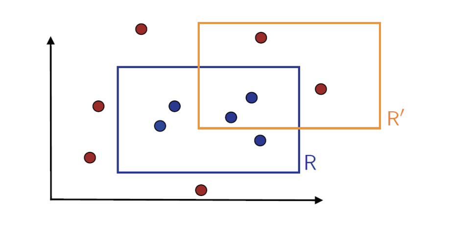
3.2 PAC-learnable? 🤔

Simplest Algorithm: I can choose the tighest rectangle R’ containing the blue points.

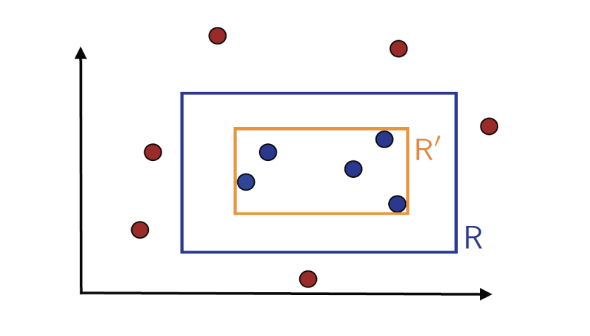
The error $\epsilon$ is the area between two rectangles R and R'

Prove:

💡 The area between R and R’ is error $\epsilon$ ❕❕❕❕❕❕

We can split the rectangle $\epsilon$ as following, and the area of the shadow is $\epsilon / 4$

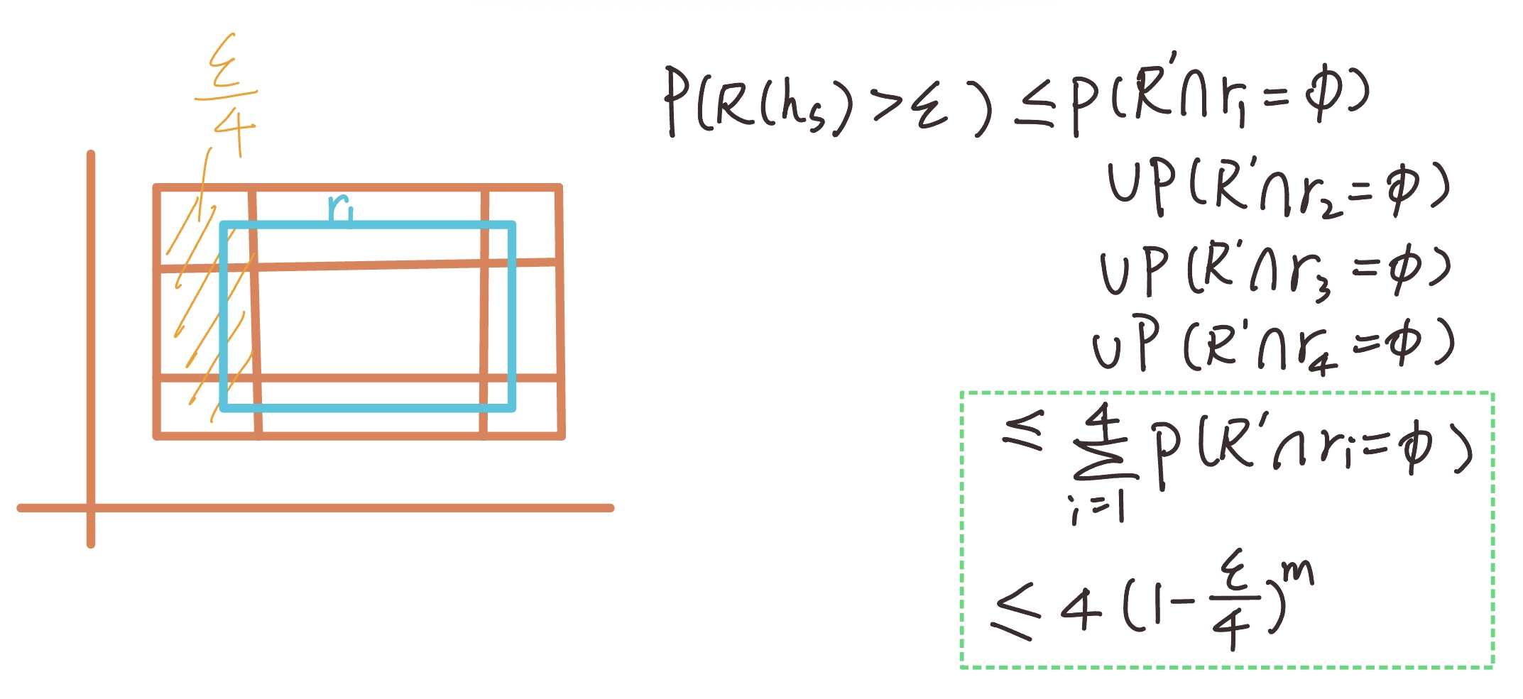
• R − R’ smaller ⇒ error smaller When the ring-shaped area between (R) and (R’) becomes smaller, the error also decreases.

• Left-hand side: $P(R(h_S) > \epsilon)$ is the probability that the error is greater than $\epsilon$. This is the same as the probability that the hypothesis fails.

  • To ensure success, (R’) must lie completely inside the border.

• Right-hand side: The worst case is when the blue rectangle (R) and the region (R − R’) have no intersection at all.

• r1, r2, r3, r4 are the four borders of the inner rectangle (R).

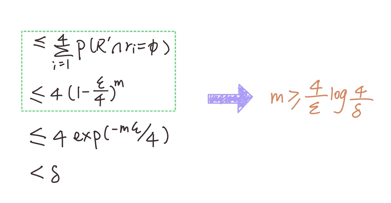
Proof of the Inequality (Green Box):

$(1-\epsilon/4)^m$ represents the probability that all (m) datapoints fall inside the boundaries $r_1, r_2, r_3, r_4$ (none of them fall into the ring $(R - R’)$, which corresponds to the worst-case scenario for the error.

Once the inequality is established, we can conclude:

$$ m \geq \frac{4}{\epsilon} \log \frac{4}{\delta} $$

To guarantee that the error is at most $\epsilon$ and the success probability is at least $(1 - \delta$ we need at least: $m \geq \frac{4}{\epsilon} \log \frac{4}{\delta}$samples.

This shows that the required number of samples grows linearly with $1/\epsilon$ (accuracy) and logarithmically with $1/\delta$ (confidence).

This means PAC definition holds:

$$ {P}_{S \sim \mathcal{D}^m} \big[ \mathcal{R}(R_S) \leq \epsilon \big] \geq 1 - \delta $$

Therefore, learning under this setting is feasible in practice.

Generalization Bound

An equivalent way to present sample complexity results is to give a generalization bound: For any δ ∈ (0, 1), the following holds with probability at least 1 − δ:

$$ {R}(h_S) \leq \frac{4}{m} \log \frac{4}{\delta} $$

• Even infinite hypothesis set is PAC-learnable for this specific example
• It is non-trivial to extend the proof to other concept classes